Pile-cap Reinforcement Design
-
Ahmed Mufty / 1 year
- 1 min read
Get the full license version now for only [product_price id = "4683"]
View If Already Paid

Get the full license version now for only [product_price id = "4683"]
View If Already Paid
Get the full license version now for only [product_price id = "4685"]
View If Already Paid
Get the full license version now for only [product_price id = "4687"]
View If Already Paid
Get the full license version now for only [product_price id = "4689"]
View If Already Paid
Get the full license version now for only [product_price id = "4692"]
View If Already Paid
Get the full license version now for only [product_price id = "4694"]
View If Already Paid
Get the full license version now for only [product_price id = "4696"]
View If Already Paid
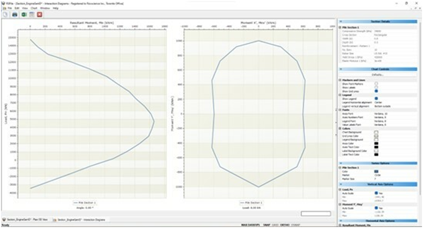
Improved Analysis of Reinforced Concrete Piles in RSPile Improved Analysis of Reinforced Concrete Piles in RSPile Published on: Oct 26, 2022 Updated on: Nov 09, 2023 9 minutes read Share: Authors: Ahmed Mufty, Senior Geomechanics Specialist at Rocscience Julien Chaperon, Geotechnical Project Manager at Rocscience Introduction This article depicts how the pile analysis under lateral loading, or couples is improved in RSPile by updating the pile flexural stiffness during the solution in cases of piles with combined flexural and axial stresses. This is raised because of the bending (flexural) stiffness of the pile varies with the level of cracking and the applied axial load. In previous versions and in most of software the bending stiffness-moment relation is a single curve constructed in the beginning of the analysis and never updated or varied along the pile length. Usually, that curve is based on the loading of the pile head while pile load may change at other depths as well, which may have significant effect on the flexural stiffness. In the latest version of RSPile release 3.014, this issue is addressed and solved. The results of the pile analysis with updated bending stiffness clearly varies with depth during the analysis. An example is solved in this article to compare the results between single and variable moment-curvature curves (bending stiffness) with depth. Theoretical background In piles with reinforced concrete sections, one of the parameters for the analysis of piles under lateral loading or bending moments is the bending (flexural) stiffness, effective EI. In ACI 318–2019, and similar codes around the world, the effective EI may be approximated by the concrete modulus of elasticity, Ec , multiplied by an effective moment of inertia Ie , a value falling between the cracked section moment of inertia, Icr , and the gross moment of inertia, Ig. Most of the pile analysis methods depend on a constant bending stiffness throughout the analysis. For LRFD analysis half of the gross moment of inertia will be acceptable and for the serviceability levels a gross moment of inertia may be an adequate value to use. With the spread of computer software for pile analysis, the bending stiffness is not constant anymore in the analysis and better value for EI is estimated during the iterations of the solution of the beam-column differential equation (by FEM or FDM methods) relating it to the last calculated curvature of the beam at that step of iteration φi where i refers to the iteration. The easiest method to calculate an updated bending stiffness for a specific point at the beam in an iteration step, (EI)i , is the relation, (EI)i= Mi/φi Derivation for this relation may be found in classical textbooks of strength of materials, see for example Higdon et al. (1978). The moment curvature curve is prepared from the beginning to pick the corresponding EI at any moment-curvature level. This helps getting better results for the response of the pile to the applied loads. The bending stiffness is highly dependent on the applied axial load at the section and the axial load varies with depth due to the soil resistance around the pile, i.e., the skin friction. The skin friction decreases the axial load with depth (or increases it in the case of negative skin friction) and it may also vary due to additional external loads applied on the pile at different depths. In traditional pile analysis the bending stiffness is taken constant along the depth which is true for elastic sections. Engineers in hand calculations or simple spread sheets assume the reinforced concrete pile as an elastic section. Meanwhile, most of the software programs the relation between bending stiffness and the bending moment in reinforced concrete sections is assumed unchanged and a single M-φ curve is used for the whole length of the pile (just like a column in a structural frame). Reese and Van Impe (2011) stated that “the errors that are involved in using the approximation where there is a change in the bending stiffness along the length of a pile are thought to be small but must be investigated as necessary”. Nevertheless, the error increases with new external loads added to the pile through the depth and in several other cases such as changes in section dimensions or materials (e.g. reinforcement ratio). This error is overcome in the recent version of RSPile 3.014. This is accomplished by generating a series of moment-curvature curves based on the range of internal axial force experienced by the pile. The bending stiffness of the reinforced concrete pile is then obtained as a function of both internal axial force and curvature. Fig.1 depicts the difference between the use of a single M-φ relation and multiple ones in the modeling. Fig.1, Representation of axial force change along the pile elements and corresponding moment-curvature curves. The single relation used is replaced with variable curves with depth. Example problem Pile section and soil model A pile with a rectangular reinforced concrete section of 500 mm depth and 800 mm width with 34 MPa concrete strength and reinforced with 10 #10 bars placed peripherally at 100mm cover. The pile is analyzed using RSPile under a lateral load in the long side direction of 150 kN applied at the pile head investigating the response applying different vertical downward loads at the top of the pile, 100 kN, 500 kN and 1000 kN. The section details are shown in the section designer of RSPile in Fig.2. Pile length is taken as 20 m fully embedded in soil. To control soil parameters effects, the soil is assumed elastic with a constant modulus of lateral subgrade reaction of 1000 kN/m3 and a skin frictional spring of 10000 kN/m3 while the end bearing stiffness is set to zero to govern the axial load distribution by the skin friction only. Fig.2, Rectangular reinforced section shown in concrete designer dialog of RSPile. Section structural capacity With the introduction of Interaction Diagrams in RSPile, users can now estimate the structural capacity of their concrete section in a single click. Fig.3 shows interaction diagram for the short column (pile), the nominal axial load capacity, Pn plotted against the nominal bending moment capacity Mn for a load applied at an angle α of 0o taken counterclockwise from x’ axis. At the right side the Mnx’-Mny’ plot
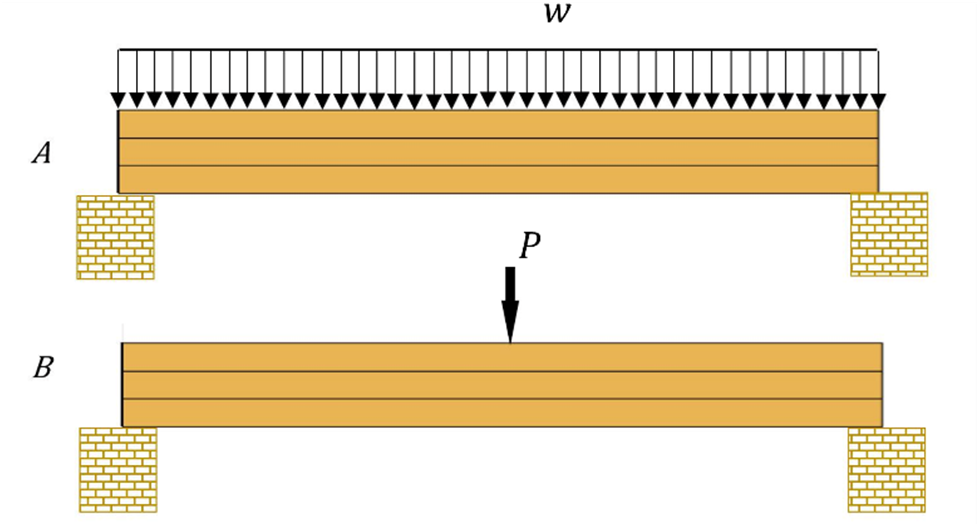
Structural Solutions by RS2 – Problem of Stacked Beams Published on: Feb 01, 2024 Updated on: Feb 28, 2024 7 minutes read Share: Author: Ahmed Mufty, Senior Geomechanics Specialist at Rocscience Introduction This article is intended to show the power of RS2 in solving a complicated structural problem. The problem chosen is the well-known stacked beams problem. It is known that if you stack identical simply supported beams made of elastic material under any distributed loading the load effect will be distributed equally to each of the stacked beams. For a simply supported beam subject to uniformly distributed load or concentrated load, the bending moment at mid-span will respectively be, M = wL2/8 M = PL/4 where, w = uniformly distributed load, units of F/L P = concentrated load at mid-span, units of F L = length of beam, units of L What happens if you have three smooth beams stacked together? For example, if you have 3 stacked beams such as the ones shown in Fig.1(a) or Fig.1(b) the resulting bending moment at the middle of the beams will be one-third of the above values. This is based on the theory of beams. But if you analyze the problem as a continuum the results will be different as the concentrated load gets distributed along the depth of the beams. The original problem A beam was subject once to uniformly distributed load w (case A) and another to a concentrated load P (case B). The load P is half the resultant of the distributed load w such that they both produce the same bending moment at mid-span, i.e., P = wL/2. A laborer got afraid of the beam failing to hold the loads. He added two stacked beams on the original beam, all symmetrical. The question is in which case will the bottom beam get less bending moment? Fig.1, stacked beams under uniformly distributed load and a concentrated load. Answer and reason: Eventually, following the beam theory, the bending moment at each beam will be equal to one-third of the original moment. Here comes the surprise: As the beam has a depth continuum theory will distribute the concentrated load and turn it from a point load at the top beam to a distributed load at the bottom beam. The answer is “Case B”. In case A, the load will be transmitted to the lower beams as is so keep the reduction in the bending moment uniform. In case B, the concentrated load gets distributed to a length that increases in the following beams and hence will decrease the moments. The distribution takes place due to the thickness of the beam (a beam with no thickness cannot distribute by thickness) and due to the subsurface reaction of the following beam (like a subgrade reaction) which arises from “springs” that can be assumed corresponding to the varying bending stiffness of the beam deflecting below the above beam. Note that, the answer is based on no friction or connection between the beams. Each beam acts individually but of course, not independently. Proof by an RS2 Finite Element Model Using the 2D FEM program, RS2, a software product of Rocscience Inc., the three beams may be modeled easily. Nevertheless, some considerations shall be taken while assigning properties to materials and interfaces. In the following, a numerical example is introduced. To simulate a model, first, dimensions and materials shall be chosen reasonably. The beam’s dimensions are taken as 22 ft in length 1 ft in width, and 0.5 ft in thickness. The material is chosen with a smooth surface (no friction material). A modulus of elasticity of 2E8 psf and a yield strength of 2E6 psf with a Poisson’s ratio of 0.25 are decided. These are given as elastic plastic material with a friction angle of zero and a cohesion of 1E6 psf in a Mohr-Coulomb model. Limit for tensile strength may be specified as well as 2E6 psf. No body forces are applied, i.e., the beams are weightless (the answer, being case B, will not get affected by self-weight addition as it is the same in both cases). The beams are stacked on two supports as shown in Fig. 2 below with a length of 20 ft between supports. The reason for not taking the supports at the ends is to show symmetric stress concentration near the supports. To separate the beams from each other, joints shall be used in RS2. This provides an interface layer in FEA. The joints shall have no shear stiffness, a very low value of 1E-12 psf/ft is used, and a normal stiffness close to the modulus of the material is used, 2E8 psf/ft. While the joints must fail in holding tension, the tensile strength of the joint is eliminated, and the shear strength is not effective as the shear stiffness is very low already. The joints are “open-ended” and have two rows of nodes. Fig.2, The beams, and the joints in RS2 Geometry. And because of numerical nature of the analysis and no lateral loads are applied, it is better to replace the hinge by rollers at the same point and on the side centers of the beams as shown in Fig.3. Fig.3, Replacing the hinge with rollers and showing the loads. Loads In Case A, a uniformly distributed load, UDL, w = 100 lb/ft is chosen, to give a bending moment at midspan of a single beam of 5000 lb. ft, and in turn, causes a tensile stress of 120000 psf as Mc/I. Hence, the corresponding concentrated load that gives similar moment and stress is 1000 lb. When the UDL is applied to the stacked three beams the bending moment is divided by the three beams equally and the resulting tensile stress at the bottom will be 40000 psf. If the results show a tensile stress at the bottom less than 40000 psf then Case B is the answer, and the proof is done. The loads are shown in Fig.3. Meshing The mesh setup in RS2 is chosen as graded mesh of 6-noded triangular elements with 400 external nodes.